PRODUCT DESCRIPTION
The LeanMan Fun with Little's Law contains several PowerPoint presentations which explain the definitions of Little's Law; provide several relevant examples to operations and finance; and suggest how to use the law to create metrics for the LeanMan Car Factory simulation exercises. Examples are included for the Learning to See the Waste and the Heijunka simulation exercises.
Little's Law Relationships provides the background of the mathematical relationship between Throughput, Inventory and Cycle Time.
Little's Law Laundry provides an interesting application of the laws in setting up a small business adventure - a laundry service.
Little's Law and Process Improvement provides an analytical approach to the LeanMan Car Factory 2-step simulation exercise where the relationships of Throughout, Inventory and Cycle Time are used to improve flow.
Heijunka and the Box takes a look at the queuing formula and the heijunka process in a mixed mode operation.
Little's Law Financial Metrics applies the law to the finance side of business, with ROAR Industries annual financial statement as a basis for the analytical look into the business performance.
John D.C. Little
Institute Professor
Professor of Marketing

John Little has had a distinguished career spanning five decades. He has published seminal papers in operations research methodology, traffic signal control, decision support systems, and especially marketing. In operations research he is best known for his proof of the queuing formula L = λW, commonly known as Little's Law.
He formed the Little's law in 1961. It states: "The average number of customers in a system (over some interval) is equal to their average arrival rate, multiplied by their average time in the system." A corollary has been added: "The average time in the system is equal to the average time in queue plus the average time it takes to receive service."
Little's Law: Inventory = Throughput × Flow Time
Where:
WIP = TH * CT
- TH = Throughput (arrival rate). This is the velocity or speed of production. It is calculated by determining how many items are produced and dividing this by the length of time it took to produce them: TH = WIP/CT.
- CT = Cycle Time (average time in the system). This is the time it takes to complete the production cycle or the average time it takes to produce one unit. Cycle time typically requires direct measurement to determine, which can be technically difficult, or it can be computed from Little’s Law: CT = WIP/TH.
- WIP = Work in Process (average number of items in a system). This is the number of items currently in production or being serviced. This figure must typically be counted directly, or can be computed from Little’s Law.
Queuing Examples:
Estimating Waiting Times: If we are in a grocery queue behind 10 persons and estimate that the clerk is taking around 5 minutes/per customer, we can calculate that it will take us 50 minutes (10 persons x 5 minutes/person) to start service. This is essentially Little's law. We take the number of persons in the queue (10) as the "inventory". The inverse of the average time per customer (1/5 customers/minute) provides us the rate of service or the throughput rate. Finally, we obtain the waiting time as equal to the number of persons in the queue divided by the processing rate (10/(1/5) = 50 minutes).
Airport Security: In an airport security checkpoint, average queue size I = 17.5 passengers, while throughput is R =600 passengers per hour = 10 passengers per minute. We want to know on average how much time a passenger spends waiting. To determine the average time spent by a passenger in the checkpoint queue, we use Little's law, I = R x T and solve for T:
T = I/R = 17.5 passengers/10 passengers per minute = 1.75 minutes
On average, a passenger spends 1.75 minutes at the security checkpoint.
Here is a sample of a Value Stream Map for a laundry process. Note that Flow Time (FT) is the same as Cycle Time in our discussion. Manual Time (MT), Automated Time (AT) and Change Over Time (CO) are not part of our laundry process. But in a more rigorous discussion using value stream mapping techniques, this added flow diagram information would provide the operations manager with a more detailed analysis ability. Non Value-Adding time (NVA) is equivalent to our laundry idle time and is added to the Value-Adding time (VA) to arrive at a total throughput of 120 minutes.
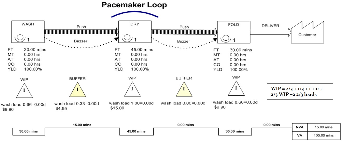
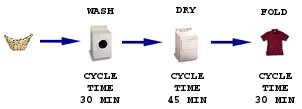
Manufacturing lead-time, or LT, is the average length of time it will take a new set of inputs to move all the way through the operation, assuming no unusual measures are taken. This is also called the throughput rate (TH) of the process stream. A load of laundry, for example, would spend one cycle (45 minutes) in the washer, including idle time, another cycle in the dryer (90 minutes total), and then two-thirds of a cycle being folded (120 minutes). The throughput rate from laundry bag to clean and folded will take an average of two hours. Note that because folding took place after our bottleneck (drying), the load didn't have to stay there for a full cycle.
The laundry example is fairly simple, but in a more complex operation it might be difficult to estimate TH at a glance. Little's Law , which is based on averages, can help. Little's Law states that:
Throughput Rate AVG = Cycle Time AVG * Work-in-Process AVG This simple rule makes sense if you imagine the path a new set of inputs (like a load of laundry) must follow in order to pass through the operation. As each unit of WIP moves forward, the new set of inputs takes its place. Each move occurs once per cycle, so multiplying cycle time times WIP will give us our total lead-time. In our laundry example, we have 2 2/3 loads of WIP. Multiplying 2 2/3 times our cycle time of 45 minutes gives us an average throughput rate of 120 minutes.
TH = 45 * 2 2/3 = 120